Radio direction finding (RDF, or just DF) is the work of finding where a radio transmitter is from the signal it emits. It's one of the oldest disciplines in electronic warfare and signals intelligence, and it's used today for everything from hunting interference near an airport to locating a drone's ground control station.
Every technique comes down to one of three measurements: how loud the signal is, which direction it comes from, or when it arrives at different places. Loudness is cheap and rough. Direction needs special antennas. Timing needs very precise clocks at several sites. Everything else is a variation on these.
Two ideas behind every method
Line of position vs. fix. Most measurements don't produce a point. A bearing produces a line, a time difference produces a curve, and a ratio of received power produces a band. Each of these is a line of position (LOP). A fix is where two or more lines of position cross, and it always comes with an error area: an ellipse, or a circular error probable (CEP), the radius of the circle that contains the transmitter half the time.
Geometry matters as much as the sensor. The same sensors give a tight fix when their lines of position cross at right angles and a long smear when they cross at shallow angles. This is GDOP, geometric dilution of precision: the factor by which geometry multiplies measurement error. Good geometry means sensors spread around the transmitter, not lined up on one side of it. Two people pointing at a sound from opposite sides pin it down; two people standing shoulder to shoulder can't.
The family of techniques
| Family | What is measured | One sensor gives | Needs |
|---|---|---|---|
| Received power (RSS) | Signal strength | A rough distance band | Calibrated receivers, a propagation model |
| Amplitude-comparison DF | Strength across directional antennas | A bearing | A directional or Adcock antenna |
| Pseudo-Doppler DF | Phase change as antennas are switched | A bearing | A switched antenna ring |
| Interferometry | Phase difference between antennas | A bearing | Two or more phase-coherent channels, calibration |
| Super-resolution AoA | The whole array's covariance | Bearings to several transmitters at once | A calibrated multichannel coherent array |
| TDOA | Arrival time difference between sites | A curve (per pair of sites) | GPS-grade timing at two or more separated sites |
| FDOA | Doppler difference between moving sites | A curve (per pair) | Moving sensors, very stable clocks |
| Single-site HF | Bearing and elevation off the ionosphere | A rough fix | An HF DF array, an ionosphere model |
Angle of arrival (AoA) is the collective name for every technique that yields a bearing: directional antennas, Watson-Watt, pseudo-Doppler, interferometry, and super-resolution methods.
Received signal strength
A transmitter sounds louder up close and quieter far away, so received power says something about distance. In practice it says less than you'd hope. Real path loss varies from any model by several decibels because of terrain, buildings, and foliage (shadow fading), and the transmitter's power is usually unknown. With typical ground conditions, a range estimate from power alone is good to about a factor of two: the transmitter is somewhere between half and twice the estimated distance.
Two refinements make power useful:
- Weighted centroid: average the sensor positions, weighted by received power. It's cheap and robust, but it can never place the transmitter outside the ring of sensors, so it works best when the transmitter is inside a ring of collectors at short range, as with Wi-Fi and Bluetooth devices in a building or compound.
- Power-difference matching: take the difference in power between two sensors, which cancels the unknown transmit power, and compare it cell by cell with the difference a terrain-aware propagation model predicts. Cells where the measured and predicted differences agree are likely locations. The result is an area on the map, and it accounts for hills and valleys because the model already knows them.
Power-based location is the cheapest method, since it works with any antenna on any radio, and the roughest: think "this neighborhood", not "this house". It breaks down with uncalibrated receivers, directional transmit antennas, and short or moving transmissions that two sensors don't hear at the same moment.
Directional antennas
Turn a directional antenna, such as a Yagi or log-periodic, until the signal peaks, or better, until it drops to a null, which is sharper than a peak. The bearing is where the antenna points. A switched-beam variant compares several fixed sector antennas instead of turning one. This is classic "fox hunting": simple and cheap, but slow, it needs a transmitter that stays on long enough to sweep, and a reflection off a building can make the strongest direction the wrong one.
Watson-Watt (Adcock) DF
Four antennas in a square, two crossed pairs running north-south and east-west, plus a central sense antenna. Each pair's output is proportional to the cosine or sine of the arrival angle, so the bearing is θ = atan2(V_EW, V_NS). The sense antenna resolves the 180° front-to-back ambiguity. Because one sample gives a bearing, Watson-Watt works on short bursts such as a one-second radio call. It's the long-standing workhorse of HF and VHF military DF, typically accurate to a few degrees, and degraded by multipath and by nearby metal that distorts the antenna pattern.
Pseudo-Doppler DF
A ring of antennas is switched in sequence very quickly, which looks to the receiver like a single antenna moving in a circle. Moving towards the transmitter raises the received frequency slightly and moving away lowers it, so the signal picks up a small frequency wobble at the switching rate. The phase of that wobble against the switching sequence gives the bearing. Only one receiver channel is needed, which makes pseudo-Doppler popular with hobbyists and public safety. It works best on narrowband FM signals with some duration, and multipath shows up as jittery bearings.
Phase interferometry
Two antennas a distance d apart hear the same wave with a phase difference Δφ = 2π·d·sin θ / λ. Measure the phase difference and solve for the angle, the same way your two ears tell left from right.
- Ambiguity: if the spacing is more than half a wavelength, several angles give the same phase. A two-element line also can't tell one side of the line from the other.
- Precision: longer baselines are more precise, and accuracy is worst when the signal arrives along the line of the antennas.
- The fix: several baselines, short ones to remove ambiguity and long ones for precision, or a two-dimensional array.
- Requirements: phase-coherent receiver channels that share one oscillator and sample clock, and phase calibration of every cable, filter, and antenna in the path.
Correlative interferometry
Instead of solving the phase equations directly, correlative interferometry (CI) compares the phases and amplitudes measured across an array against a stored table of what that array produces for every frequency and direction. The table is measured in advance on an antenna range or on the vehicle itself, so it already includes the array's imperfections and the effect of the vehicle's metal and mast. That makes CI accurate and robust, often around a degree in good conditions, and it's common in commercial and military DF systems. The cost is building the calibration table for every array and platform.
Beamforming and super-resolution
With many coherent channels, an array can listen in every direction at once.
- Beamforming electronically steers the array and measures power in each direction. Its resolution is about the wavelength divided by the array size, so two transmitters closer together than that blur into one.
- Capon (MVDR) is adaptive beamforming with sharper peaks.
- MUSIC separates the array covariance into signal and noise subspaces and finds the directions orthogonal to the noise. It can resolve up to one fewer transmitter than it has channels, on the same frequency, beyond the beamwidth limit.
- ESPRIT uses the shift between two identical sub-arrays and needs no search.
These methods are powerful but sensitive to array calibration, to the number of samples, and to coherent multipath, where reflections look like extra correlated transmitters.
TDOA: time difference of arrival
Two separated sites timestamp the same signal. The time difference fixes the range difference, c·Δt, so the transmitter lies on a hyperbola with the two sites as its foci. Three sites give two independent curves that cross at a fix, and more sites over-determine it.
- Ordinary antennas: TDOA works with omnidirectional antennas, with no array and no phase calibration. That's its big advantage.
- Timing is everything: 1 ns is about 0.3 m of range difference, 100 ns about 30 m, and 1 µs about 300 m. Every site needs a GPS-disciplined clock and hardware sample timestamps, plus a plan for when GPS is jammed.
- Bandwidth is everything: timing precision improves with signal bandwidth and with signal-to-noise ratio times duration. Wideband signals such as data links, LTE, and drone video locate well. Narrow 12.5 or 25 kHz push-to-talk voice doesn't, unless it's captured for a long time.
- Geometry: TDOA is best when the transmitter is inside the polygon of sites and poor along the extension of a baseline.
- Backhaul: sites have to share the same snippet of raw signal (I/Q) or correlate against a common reference, which costs bandwidth and is itself an emission to manage.
With only two sites, TDOA gives one curve: a line of position to combine with a bearing or a power-based area.
FDOA: frequency difference of arrival
When sensors move, each one sees a Doppler shift that depends on its velocity towards the transmitter. The difference between two sensors defines an iso-Doppler curve, and combined with TDOA from the same pair, a single snapshot can give a fix from just two platforms. FDOA is an airborne and satellite technique: it needs moving sensors with well-known velocity and extremely stable clocks, since 1 Hz at 1 GHz is one part per billion and the whole Doppler shift at 1 GHz and 50 m/s is at most about 167 Hz. Ground sensors that don't move produce no useful FDOA.
Single-site HF location
At HF, signals bounce off the ionosphere. An array that measures both the bearing and the elevation angle, combined with a model of the ionosphere's height, turns elevation into range and gives a fix from one site. Accuracy is a few percent of range at best. It's a long-range, low-precision technique for shortwave only.
Combining measurements
Every method produces lines of position with errors, and no single clue is perfect. A good system combines all of them, and bearings, time-difference curves, and power-based areas each shrink the answer. Even "this sensor did not hear it" is evidence. The combined solution is a fix with an error ellipse, and a fix with good enough kinematics becomes a track that other sensors (cameras, radar, acoustics) can use to look in the right place.
"RF fingerprinting" means two different things, and they're often confused. Location fingerprinting matches live signal strengths against a pre-surveyed map. Emitter fingerprinting identifies an individual radio from the quirks of its hardware. The second is identification, not location.
Rules of thumb
These are for planning, not promises.
| Quantity | Rule | Example |
|---|---|---|
| Bearing error to cross-range error | About range × error in radians | 1° at 10 km ≈ 175 m; 5° at 10 km ≈ 870 m |
| Two-bearing fix | Best when bearings cross near 90° | Shallow crossings stretch the ellipse along the line of sight |
| TDOA timing to range difference | Speed of light × timing error | 10 ns ≈ 3 m; 100 ns ≈ 30 m |
| RSS range | Multiplicative error, not additive | 8 dB shadow fading on the ground: about ×1.85 |
| Interferometer | Unambiguous if spacing ≤ half a wavelength | At 300 MHz, spacing ≤ 0.5 m |
| Array resolution | About wavelength ÷ array size, in radians | 300 MHz, 2 m array: about 29° |
Everything degrades with multipath, low signal-to-noise ratio, short transmissions, frequency hopping, and directional transmit antennas. And no RF technique can find a transmitter that isn't transmitting: many one-way attack drones fly preplanned GNSS routes in silence, and finding them takes radar and acoustic sensors.
Where Empyrean fits
Location is only useful when it reaches the people making decisions, alongside everything else they can see. Empyrean puts RF observations on the same operational picture as tracks from radar, cameras, ADS-B, and Remote ID, so an emitter location is a cue for other sensors rather than a dot on a separate screen.
Today, Digital Force Protection locates Wi-Fi and Bluetooth devices from two or more collectors and shows each estimate with its confidence ellipse.
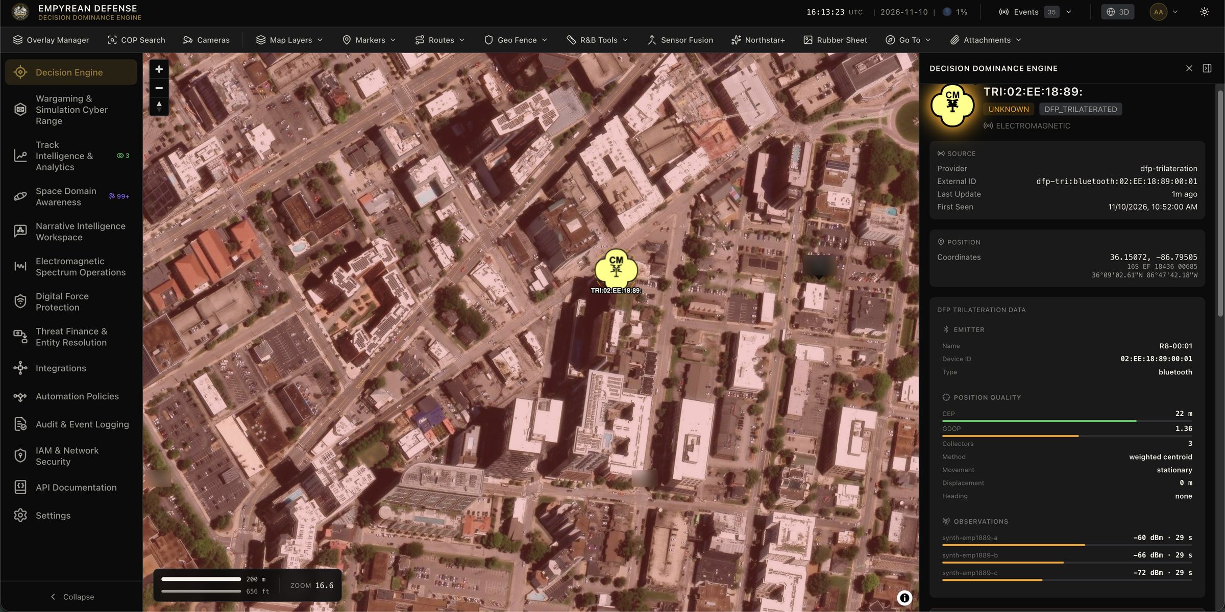
Spectrum collection, emitter detection, and signal classification run in the EMSO workspace across the supported SDRs.
Going deeper
- What is EMSO? covers the wider discipline that direction finding sits in.
- What is Sensor Fusion? covers turning fixes and bearings into tracks.
- Sense, Make Sense, Act: How to Conduct Counter-UAS covers where RF detection fits among the other drone sensors.
